Export Maps with Data to Google Earth
In Scan/US Version 8, you can create ring areas, polygon areas based on driving time, as well as groups of ZIP codes, microgrids, or anything else.
You can export all of these to Google Earth. There are two basic ways to do this.
Method 1: Select object, then right-click and choose "Locate in Google Earth"
Method 2: Select Object(s) in Object Manager, then from the Export button at the bottom of Object Manager, choose "Export Objects" OR Locate in google Earth
Variations on these techniques give you a wide range of map output possibilities.
Note: On some computers, Google Earth offers a choice of "renderer". When using the DirectX renderer, your layer may not appear. If this happens, try the OpenGL renderer (or decline the DirectX option when offered a choice), to see your exported map layers.
Method 1: Select Object, Locate in Google Earth
This method works with any object you can select in Scan/US.
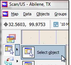
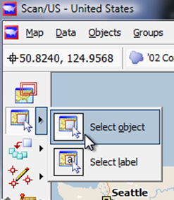
First, make sure you are in Select Object Mode:
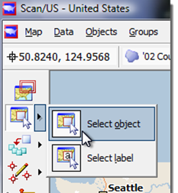
Select Object mode
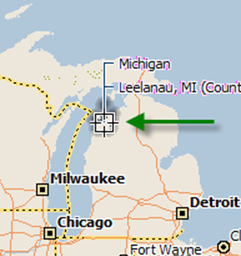
Then, with the map of the United States showing, click on (for example) Leelanau County Michigan. The geographic object choice tree for that location appears. Here it shows the state and county. Depending on where you click, it would show objects on other layers.
image
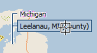
Leelenau County
Select the county name, and the county will be highlighted, as above left. Several islands are within the county, which you can see highlighted below.
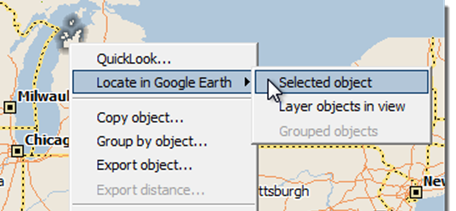
Right-click to get 'context menu'
Finally, as above, right-click your mouse on the highlighted Leelenau County, and the right-click "context menu" appears. When you choose "Locate in Google Earth" from the right-click context menu, you see two more options: Selected Object, and Layer Objects in View.
When you choose Selected Object, The Windows application Google Earth will start, and the Google globe will spin to Michigan. Leelanau County will be shown, as below. Note: Google Earth, a free download from earth.google.com, must be installed on your computer in order for this to happen.
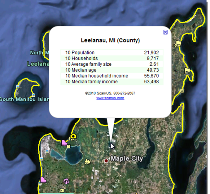
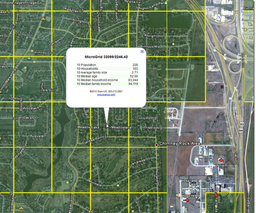
Leelenau County, Michigan, showing demographic numbers
Notice in Google Earth that when you click anywhere within the yellow-bordered area of Leelanau County, Michigan (or whatever county you exported to Google Earth if you clicked on a different county to begin with), the values of demographic data items appear in a pop-up window, with the Scan/US phone number and link to the Scan/US website, www.scanus.com.
It's worth noting that when you run this example, your demographics will be the Scan/US 2012 estimates, or whatever the current year is for your subscription.
These demographic data items were exported from Scan/US, based on the demographic data items you checked off in the Scan/US Quicklook dialog at the time of export. Let's do the same thing with a polygon you create, based on a 15-minute driving time, centered on downtown Abilene, Texas.
First, make sure you're in Framing mode. Click the Framing mode button at the top left of Scan/US, just underneath the latitude-longitude readout.
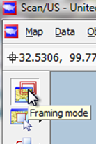
Framing mode
Then, draw a rectangle to frame the Abilene vicinity. A number appears as you draw the rectangle (green arrow), indicating the height of the new study area.

area height
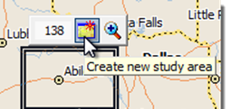
Create new study area
When you have drawn the rectangle, a button panel appears. Choose "Create new study area" . The New Study Area dialog appears.
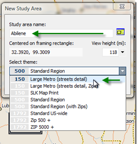
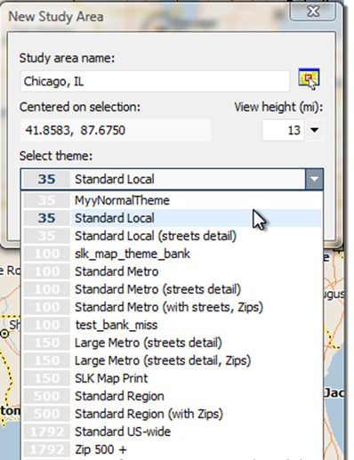
New Study area: name it and choose a theme
Type in a new name such as "Abilene Area", and choose a theme from "Select Theme", such as "Large Metro" (green arrow) . You may wish to zoom in closer, using the ZOOM SLIDER (shown below at left by the green arrow).
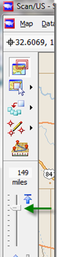
Zoom Slider (the mouse scroll wheel will also zoom)
After zooming in on the center of the new Abilene study area create a Drivetime area. From the Objects Menu, select "Create layer", and choose "Areas..". The Create Layer Areas Dialog will appear.
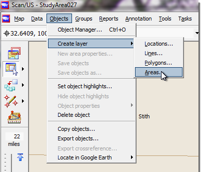
Create layer on Scan/US Objects menu
When the Create Layer Areas dialog appears, you will NAME the new layer, CLICK the TAB that says "DriveTime", and enter a number for the drivetime - 15. Then, after you click OK, anywhere you CLICK in the map, a New DriveTime area will be created, and you will name that area. In this example, we make two, Abilene, and Sweetwater.
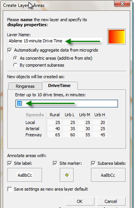
Create Layer Areas: DriveTime Tab
The name you give the layer is the name which, from now on, appears in the Map Layers dialog. Give it a good name! Here we have given the name Abilene 15-minute, but a better name would be "15-minute Drivetime Areas".
Notice the checkbox underneath the name, next to "Automatically aggregate data from microgrids". Checking this box makes Scan/US summarize the demographic values of the 15-minute. Leave it checked.
This dialog can also be used to create concentric rings, by choosing the "Ringareas" tab. Ring areas can be exported to Google Earth, too. If you don't want your new site to be labeled, or marked with the site marker, you can un-check the boxes at the bottom, and they won't appear. Here we leave them checked.
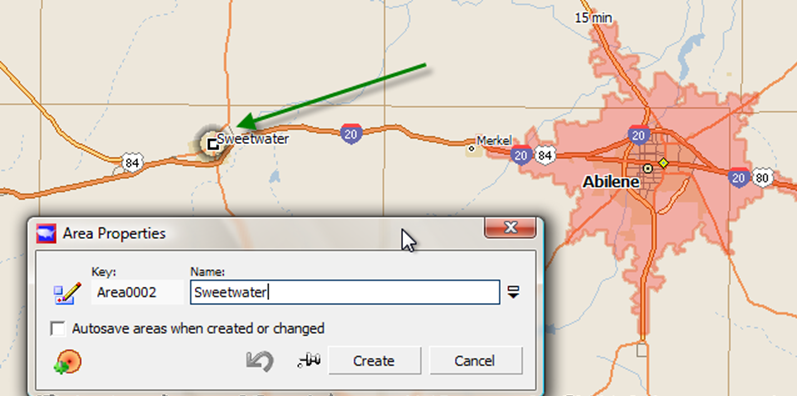
Area Properties after clicking on Sweetwater
After you click in downtown Abilene to create a drive-time polygon there, click on Sweetwater, a small town to the West, and make another drivetime polygon. The Area Properties Dialog will pop up, and give you an opportunity to type in a new name. Type in the name "Sweetwater 15-minute drivetime".
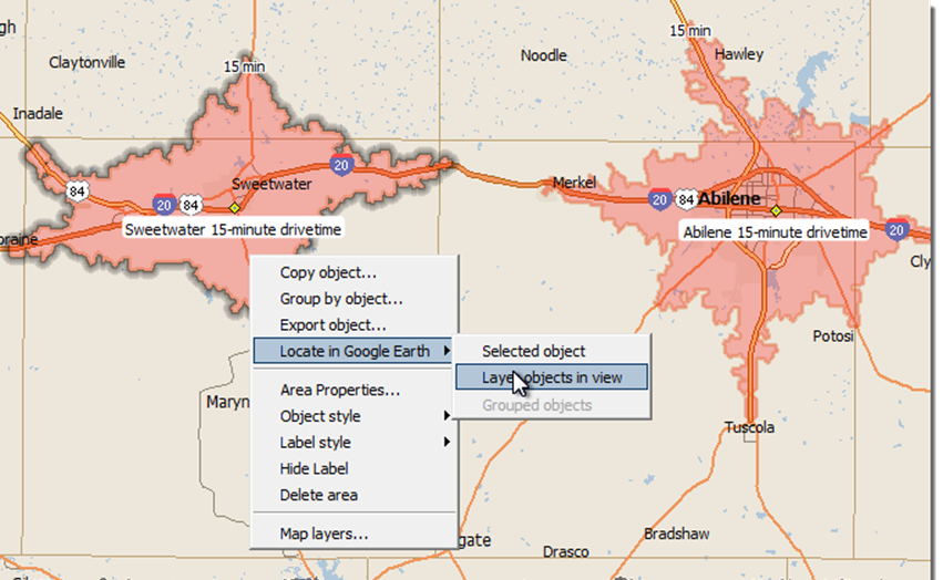
Right-click the drivetime object to get the context menu
Now when you right-click on the selected object - the Sweetwater 15-minute drivetime -select Locate in Google Earth*, and chooseLayer Objects in View*, in order to export BOTH drivetime areas.
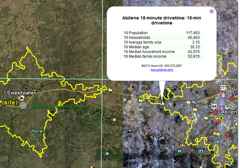
Abilene and Sweetwater Drivetimes with demographics
In Google Earth, you will notice the center of the drivetime area marked by a bullseye symbol. Clicking inside the drivetime area shows the exported demographics for the area, which were automatically summarized by Scan/US, and which can also be viewed back in Scan/US by selecting "Quicklook" from the Scan/US Data menu.
Export Microgrid thematic map to Google Earth
Now that we have exported a pre-existing county boundary, and two created drivetime areas to Google Earth, in the last example of part 1 we will make five groups of Scan/US Microgrids in the Abilene 15-minute drivetime area, corresponding to different income ranges of 2010 Median Household Income.
Then, we will export these groups to Google Earth using the Grouped Objects option of Locate in Google Earth.
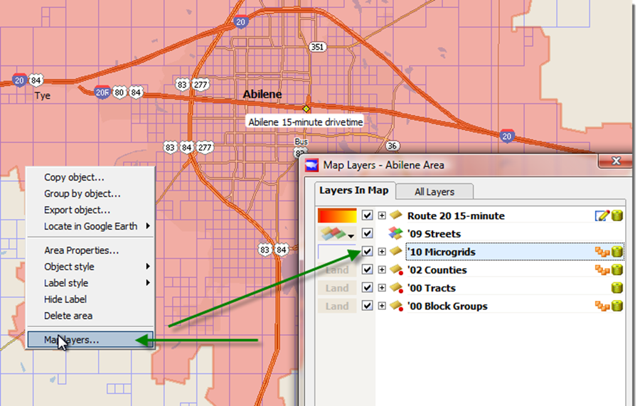
From the context menu, right click and choose Map Layers. The map Layers Dialog appears. Click the checkbox next to '10 MicroGrids - on your map it may say '11 MicroGrids, and the Scan/US MicroGrid layer will appear.
image
Now, use "Group by Object" on the Groups menu to narrow the number of MicroGrids to the total number contained just within the 15 minute drivetime of Abilene.
From the Groups menu, choose Group By Object, and make sure Abilene 15-minute drivetime is selected as the "Overlay layer" (green arrow):
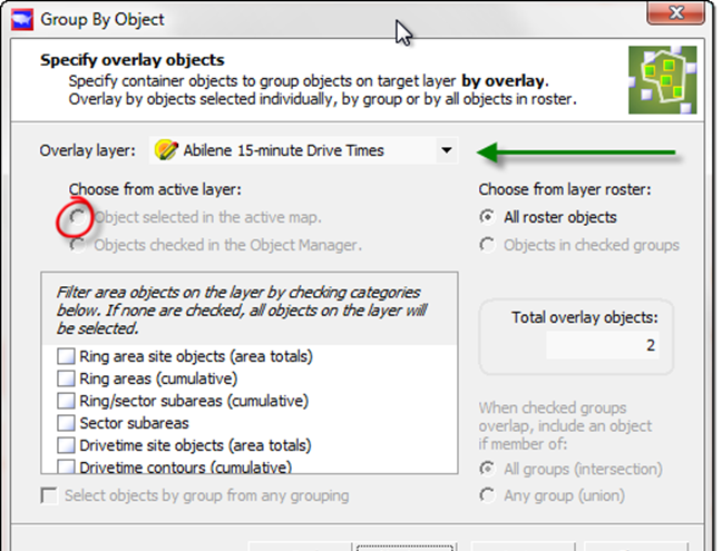
Group By Object
Notice that you may not be able to pick the option you really want to, which is "Object selected in the active map." In order to choose this object, an object must be selected in the map.
Select Object
First, make sure you are in Select Object mode
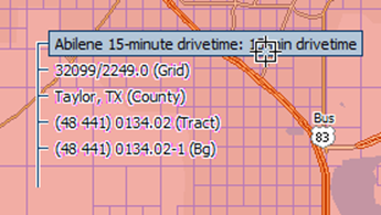
Click in map: Object selection "tree" menu appears.
Click anywhere within the Abilene 15-minute drivetime, and click on "Abilene 15-minute drivetime" in the object selection menu to select it .
Now your Group by Object Dialog will look like this, with just one object selected (red circles below).
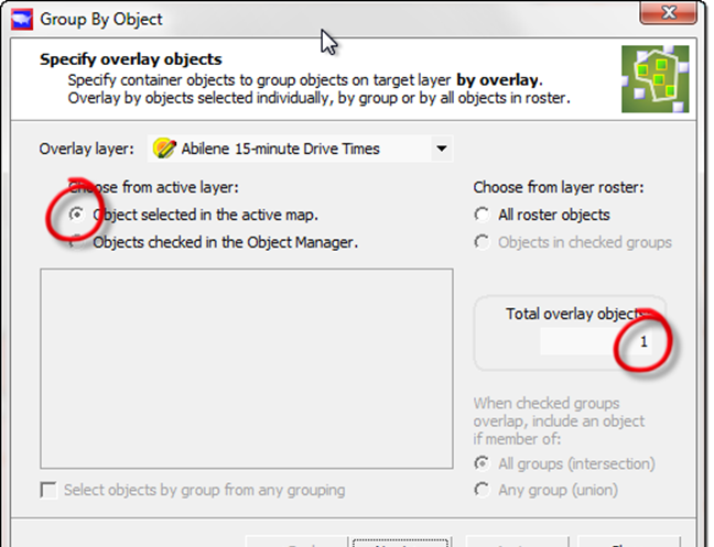
Group by Object: 1 object selected
Click "Next" to choose the target layer you will group - in this case Microgrids.
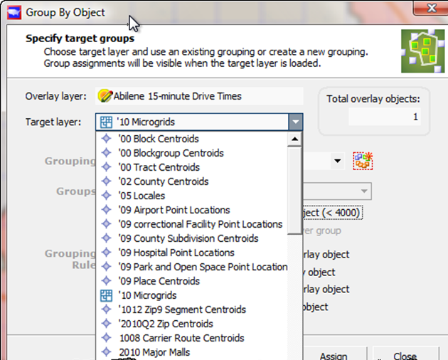
Group by Object: Specify target groups.
Now that you have an overlay and a target layer, are you ready to hit "Assign?" Not quite:
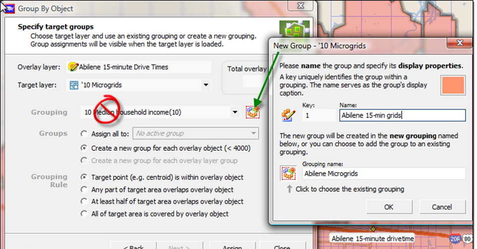
Make sure to make a new grouping!!
You don't want to add to the existing grouping (red no-no circle).
Instead, create a new grouping by clicking the New Grouping button (shown by green arrow). Give comprehensible names to the new group and grouping so you will understand what you're doing in the next step! Then click OK in "New Group", and Assign in "Group By Object". This will color in the microgrids a similar orange color as the drive time area.
Let's change the MicroGrid color to a more-prominent blue. From the Groups menu, choose "Group Manager", and click on the color patch to the left of the group "Abilene 15-minute drivetime". This brings up the Area Style selector, where you will choose a new color, and click Apply. The Microgrids are now blue.
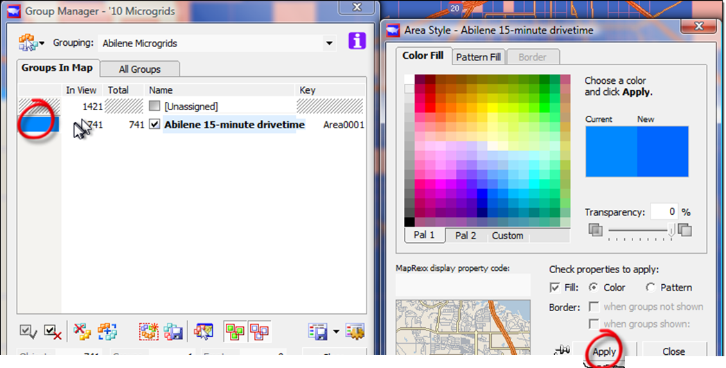
Group Manager showing one group, customizing the color
Now to narrow down the selection of grids from a couple thousand to about seven hundred.
From the Objects menu choose Object Manager, and click the menu "Select by subset" in the upper left hand. It may not look like a menu, but the little black triangle means that it is one.
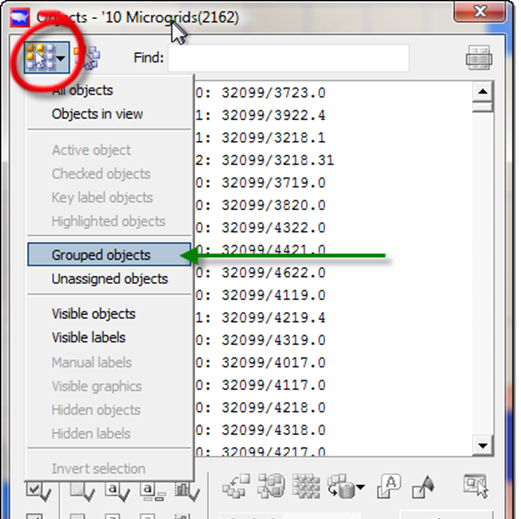
Object Manager: "Select by subset" menu
Choose Grouped objects, and you will get the following: all the grouped grids selected
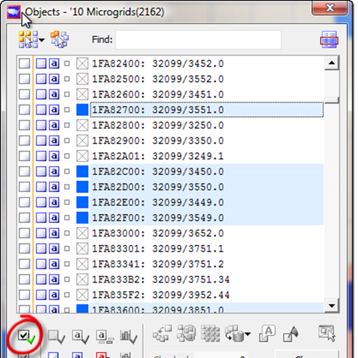
Light blue highlighting showing selection
Object Manager works by first selecting objects, then checking them. Give the selected objects a check by clicking the green checkbox in the lower left corner of Object Manager (red circle above).
Classify by Value
NOW we are ready to do a thematic map of2010 Median Household Income on the grids.
From the Scan/US Data menu, choose the first item, "Classify by value.."
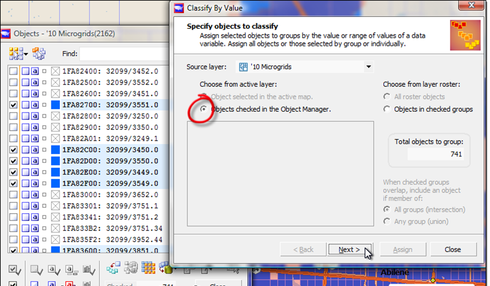
Classify by Value Dialog
Because you have just assigned checked the grids based on the group, Objects checked in the Object Manager (red circle) is already checked. Just go ahead and click Next, where you will specify the grouping variable.
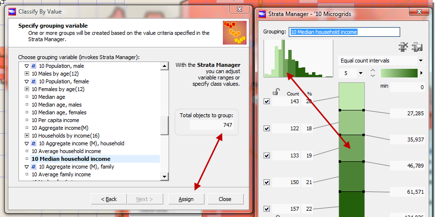
Classify by Value: Specify grouping variable
Once you choose the variable "10 Median Household Income", Strata Manager pops up to the right, and divides the grids into 5 groups, with the income ranges shown on the right. Each group has roughly a fifth of the total number of grids, shown in a column under "count" on the left. When you click "assign", in the Classify by Value dialog, the grids will be colored in shades of green according to the value of the median household income in that grid.
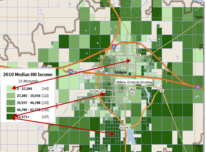
Classify by Value -- arrows show MicroGrids depicted in legend
Notice the low-median-income area north of the center of town, a high income area southwest of the city center, and another high-median-income area just to the west of where 83/84 heads due south. This third area is where we will zoom in with Google later on. Select a grid, right-click for the context menu, and choose "Locate in Google Earth" again, this time you will see Grouped Objects as an option.
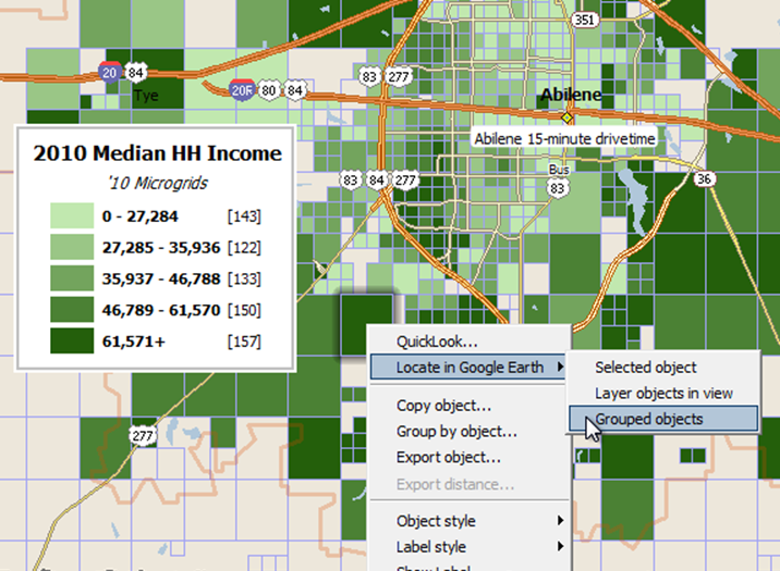
Right-click, locate in Google Earth, Grouped objects
Choose Grouped objects, and 'let the great world spin'. The next screen capture of Google Earth shows an overlay of the dark green Scan/US MicroGrids - in this case the median income range of over $61,571 - atop the streets of the subdivision in question, and one grid in particular has been clicked on: values for all the different grids are now clickable on your Google Earth.
Median household Income Grids in Google Earth
This completes the three options of Method 1, Locate in Google Earth. You may have noticed another option on the right-click menu, "Export Object", which allows you to export both .kml and .kmz files, which are filetypes recognized by Google Earth, as well as .shp shape files, recognized by ArcView. These all work perfectly well, but they do not start up Google Earth after export, so they are less suitable for an interactive demonstration. However, if you want to send an overlay file to someone else who has Google Earth installed, these file formats are ideal for that purpose.
We now proceed to Method 2: Select Object(s) in Object Manager, then choose "Export Objects" OR Locate in google Earth
Method 2: Select Object(s) in Object Manager, Locate in Google Earth .
Let's say, for the purposes of this example, that we want to find and look at two adjacent ZIP codes in the Chicago area that have very large families. (We don't know in advance which ZIP codes we are going to use). Our business model involves some kind of family-related product or service. And we want to see where within the ZIP code the large family households are concentrated.
Here is the summary of our process: Using Classify by Value, we will make a MicroGrid-based thematic map of the Chicago area. We will narrow the focus with Strata Manager to show only those grids with high family values.
We will choose which ZIP codes to use, based on where the high-value grids are. Then, because grids in this group are spread all over Chicago and we can only bring our business resources to bear on a smaller area of roughly 2 adjacent ZIP codes, we will use Group by Object to create a group of grids that fall just within the two ZIP codes. To do this we will make a small "group" of just those two ZIP codes, and use those two ZIPs as a template to gather the grids that fall within them into another group. Then we will export those grids to Google Earth and have an aerial look at the residential buildings in the area.
First, make sure you are in Select Object Mode:
Select Object mode
Click on the city of Chicago, and select Chicago, IL from the object selection tree:
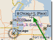
Choose Chigago, IL (Place) using Select Object
From the Select Theme dropdown, choose the theme called Standard Local. It does not have ZIP codes, and so you can see how to add a ZIP layer from the Map Layers Dialog. Normally you would choose a theme from this list that has ZIP codes already in it.
Choose a theme: Standard Local. Add ZIPS later.
When the new Study Area is formed, from the Map menu, choose Map Layers.
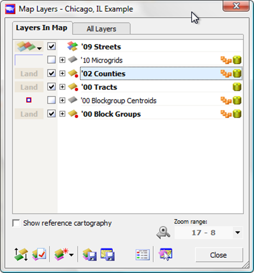
Map Layers shows what's in the map.
Notice that you don't see ZIP codes in the list yet.
We will do three things: add ZIP codes, turn on MicroGrids, and turn off Streets. Click the All Layers Tab. This shows the "palette" of all the layers that you can put in the map. Scroll the list down to Postal Geography, and click the little "plus" sign to expand the postal options.
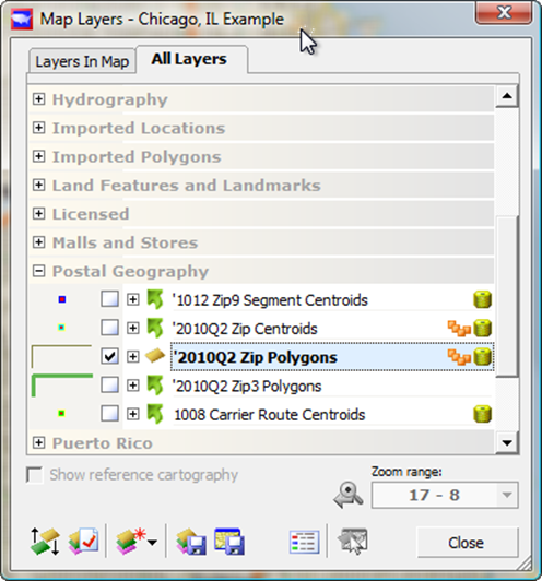
Select 'All Layers' tab and choose ZIP polygons
Once you have expanded Postal Geography you can see the possible layers. What are these layers?
Zip9 Segment Centroids are the point locations for Zip+4 Centroids, here referred to as Z9's because 5+4=9.
Zip Centroids are the center point location for each ZIP code.
ZIP centroid weighting: In general the zip centroids are carrier route centroids weighted by delivery counts. In cases where data is incomplete, the centroids might be geographic centroids, post office centroids or manually placed centroids. Carrier Route centroids are weighted by street address ranges delivery counts.
The third layer you could add is 2010 Zip Polygons from the 2nd Quarter (because ZIP codes change constantly we make a new file each quarter - by the time you do this example the number could be different).
Finally are two layers you may never have heard of: Z3 polygons which are areas corresponding to the first three digits of the ZIP code, and Carrier Route Centroids. These are point locations corresponding to the middle of the walk route that a postal carrier takes when he is delivering your mail.
Each of these areas have demographic data attached to them, but we are only interested in the borders of the Zip Polygons, so check the checkbox as pictured above.
Then, click the Layers in Map tab of Map Layers to return to current-map control.
With the "Layers in Map" tab once more active, you will see the ZIP layer checked and at the top of the list of layers in the map. And if you look closely in the map, you may be able to see faint green lines indicating the edge of the ZIP codes. To the left of the checkbox (red circle) that determines the appearance of ZIP polygons in the map is a green line indicating the boundary color - this green line is also a button, which you press. When you do, the Area Style selector will appear, as shown below. A variety of line styles appear for you to click, and you can also adjust the Transparency slider to the right, making it less transparent (more visible). If the number shown below as 84 (red circle) is changed to zero, it will be fully non-transparent, in other words opaque. Slide it all the way to the right.
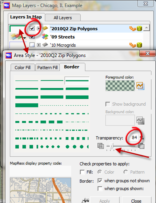
Choose 'Area Style', and move transparency towards zero (opaque).
When you slide the transparency slider back and forth, the Foreground color "well" above it will change, showing the old color and the new color next to each other. When you are satisfied that you have what you like, click Apply. You will see a map similar to the next one.
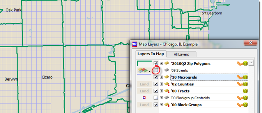
Turn off streets by clearing the streets checkbox (red circle above)
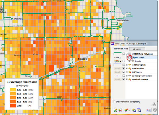
In order to create a clear view of our upcoming group operations, click the Streets checkbox off (red circle), and turn the MicroGrids on, as shown above. If you want to view the ZIP code numbers, expand the "plus" sign next to the ZIP polygons layer, and click on the checkbox for the labels. The ZIP numbers will display, except when pushed out of the way by an existing town label, such as Cicero.
Now from the Data Menu, choose Classify by value.
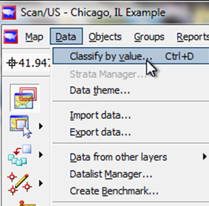
Data Menu: Classify by Value
The following pair of dialogs appear:
Object Manager, Select by subset
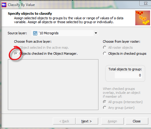
Classify by Value, Object Manager option
The two dialogs shown above are Object Manager (top) and Classify by Value (bottom). If Object Manager does not appear, make sure the "Objects checked in the Object Manager" button is selected (red circle).
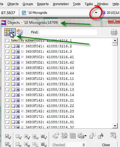
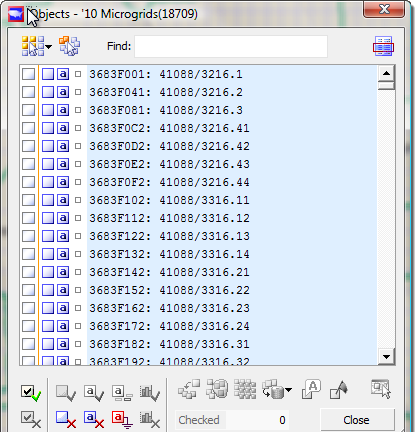
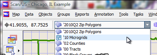
When Object Manager appears, its title bar will say something like '10 Microgrids(18709). The '10 represents the year of the grids and the 18709 is the number of grids in the map. Yours might say '13 or '14 Microgrids (19853) if you have a larger map, or some other number of grids. If it does NOT say grids, then you need to adjust the layer using the layer dropdown shown above at the top of the map (red circle). Once it shows grids, there will be a list of all the grids in the map, with their alphanumeric key names. You will never need to know the exact name of any particular grid, but there they are, identifying the grid uniquely among all two-and-a-half million grids in the US. Just in case.
The two controls in the upper left of Object Manager are pictorial buttons for two menus, Select by subset and Select by group.Press Select by subset.
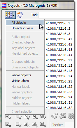
Select by subset menu, Object Manager
Here is how Object Manager works: first you select objects, and then you check them on and off using the two checkboxes at the lower left. Once they are checked, you can control their visibility, label visibility, etc, with the other controls on the bottom. The combination of selection and checking is very easy and non-error-prone, combining ease of selection highlighting with semi-permanence of checking. In this example, just choose "All objects", and the objects will highlight, as in the next capture:
Object manager, all objects selected
Then, check off the objects with the green checkbox at the lower left. Object Manager will appear as in the next capture:
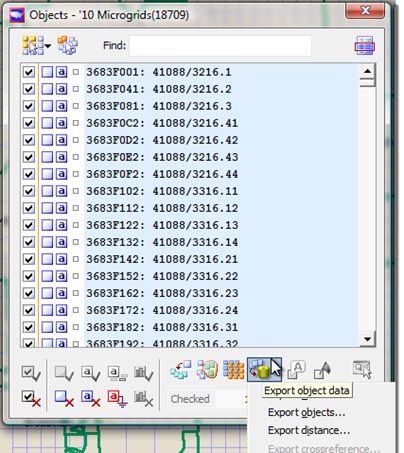
Checked objects, ready to Export object data
At the bottom left, notice that the green check checkbox is grey, and the red X is live - now you can un-check those boxes if you need to.
On the same line, it will say checked 18709 objects. Later you will return to press the "Export objects" button, shown pressed, and select "Locate in Google Earth". DON'T PRESS IT YET: it would export ALL the grids, not just the ones grouped by two ZIPs. You can also see several other export options, which we don't need for this example.
Now that you have got your selection, press the NEXT button. In the list underneath "Choose grouping variable", select the 10 Average family size.Strata Manager will pop up. Notice the panel, "total objects to group 18709". When you press "Assign" all the grids will be filled with a color according to the value of Average family size for the grid. In Strata Manager the Count column on the left side of the box shows the number of grids in each value range.
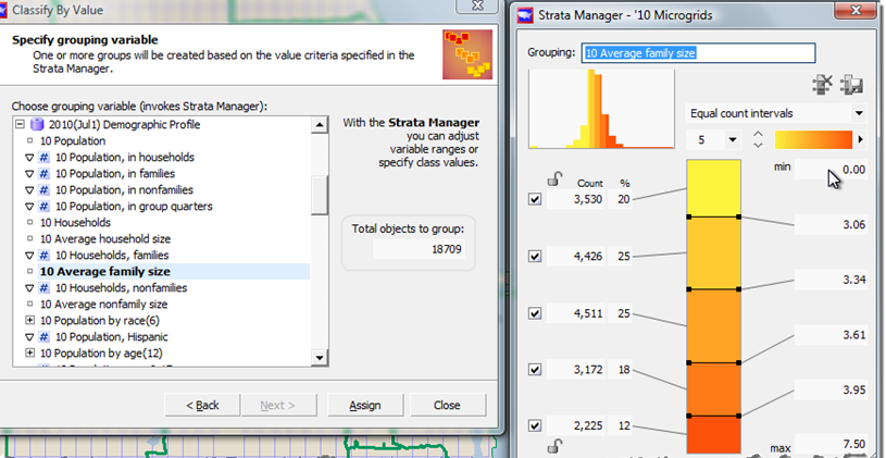
Classify by Value, specify 'grouping' variable
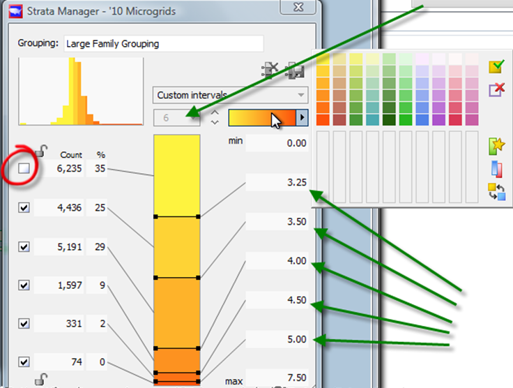
Notice, above, in Strata Manager, the blue-outlined default Grouping name "10 Average family size". Change this to the name you want to see in the grouping legend in your map. For example, "Large Family Grouping". If you want to change the grouping colors, click on the color ramp (white arrow) to expand the choices. Choose a different color row and click the green checkmark to make it take effect.
The good old Scan/US Strata Manager!
Change three other controls to show a concentration of large families by grid. First, change the number of intervals to six (single green arrow). Second, edit the range values to show closer range limits at the upper end (five green arrows). Notice how the columns showing the count of Microgrids and their percentage of the total change values, giving you a preview. Third, uncheck display of the lowest range (red circled empty checkbox). The bottom 35 percent of your range, grids where family households have an average of 3.25 members or below, will not be colored in at all. Finally, click "Assign."
Scan/US MicroGrids by average family size
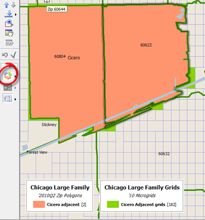
You can see that two ZIP codes, 60804 in Cicero and 60623 to the east of it, are nearly half full of grids with an average family size of at least 4.5. But .. how do you know those ZIP numbers? In Map Layers (either right-click on the map screen or choose from the Map Menu), expand the ZIP polygon layer to show "Object labels" by clicking the "+" sign next to ZIP Polygons. Then you can check the Object labels checkbox to turn on for ZIP codes.
Zoom slider to zoom in
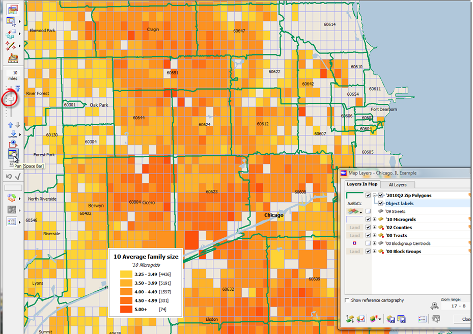
In order to see the ZIP code label appear next to Cicero, you may need to zoom in using the zoom slider (circled in red). After you have zoomed in, you can pan the map using the control with the little hand just underneath the zoom slider, called Pan (Space Bar), because it can also be activated by tapping the space bar on your keyboard. In "pan mode," the mouse cursor turns into a small hand, and you can reposition the map so the two ZIPs in question are in the center. When you are done panning, turn pan mode off by clicking the Pan (Space Bar) button again.
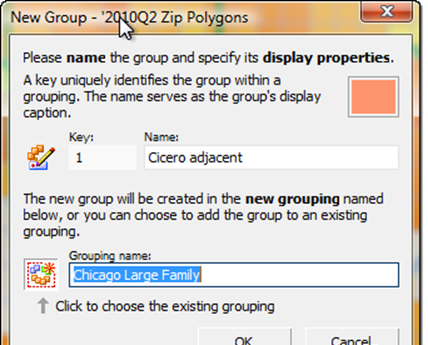
Now it's time for our grouping hop-skip-and-jump. From the Groups Menu choose New Grouping.. Give your grouping the name "Chicago Large Family", in case you want to look at ZIPs in other areas of Chicago, and call this particular new group Cicero Adjacent. Click OK.
New Group
As you do this, make sure that Zip Polygons are the current layer. It will say New Group - '2010Q2 Zip Polygons in the title of the dialog (white arrow).
When you click "OK" it will create a new group, and put you into "Assign object to group" mode. Double-click on ZIP 60804 and it will be assigned to the new group, "Cicero adjacent." Your map will look like this:
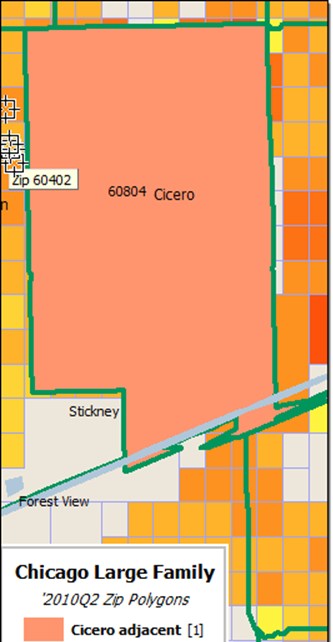
First ZIP added to group "Cicero adjacent"
Notice the "1" next to the name of the group, indicating that you have added one ZIP object to it.
Repeat the double-click on the adjacent 60623, and when your map looks like below, from the Groups Menu choose Group By Object .
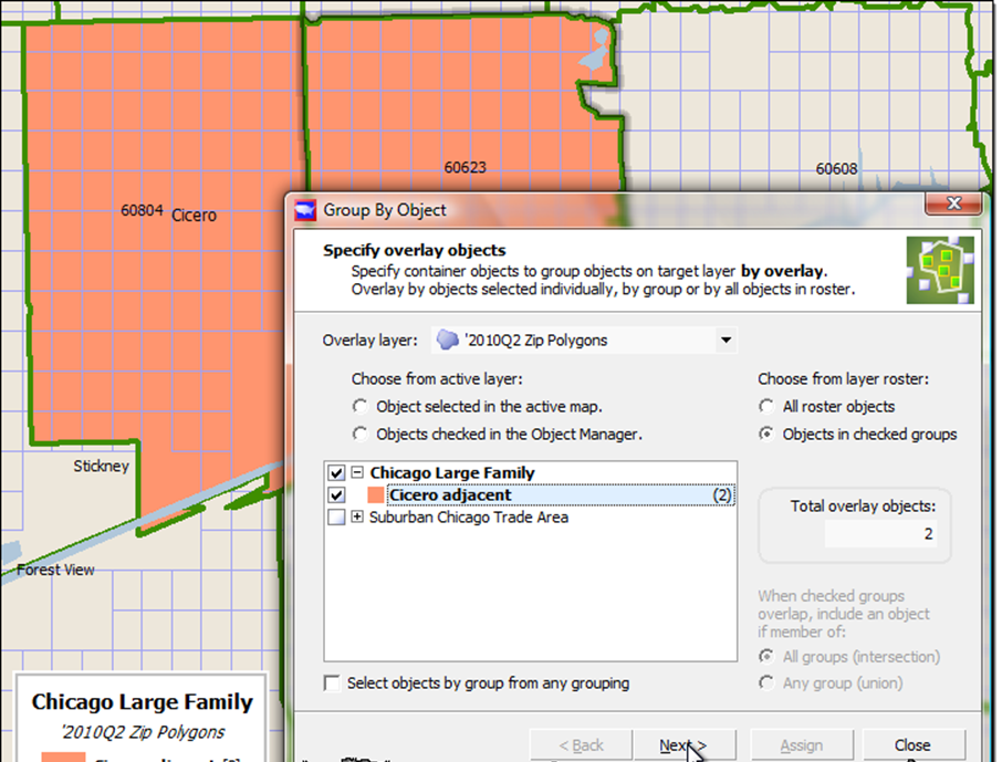
Group by Object: Specify overlay objects
Click the "Objects in checked groups" button in the right column, and check "Cicero adjacent" from the list of possible groups. Notice that the Overlay layer is your ZIP polygons layer. The "overlay" layer is the "group by" layer. It will always show the total number overlay objects, in this case "2"
Click "Next" to go to the next step, where you will choose the target layer of grids, and define a new group to put them in.
Notice (below) that there are three ways to assign groups. Click to select the third, "Create a new group for each overlay layer group." There is just one overlay layer group, and you are going to create one group, so this option is the correct option to choose for the goal of this exercise.
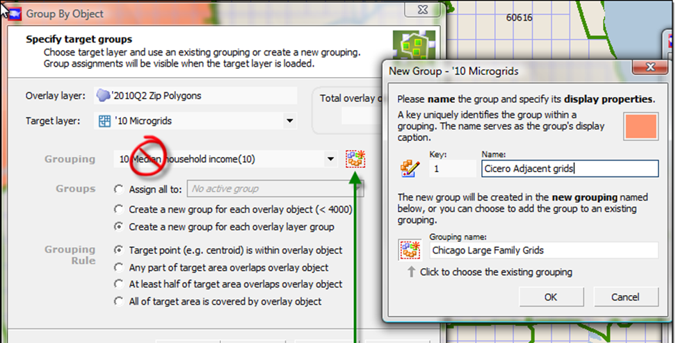
Specify target groups
Typically you will NOT want to assign it to the current grouping (red no-no circle). Instead, click the New Group button (green arrow) next to the Grouping dropdown to create a new Group and Grouping. Fill in "Cicero Adjacent Grids" for the group and "Chicago Large Family Grids" for the grouping. And, just to make it clear which layer is which, grids vs ZIPs let's change the orange color of the new grid-based grouping.
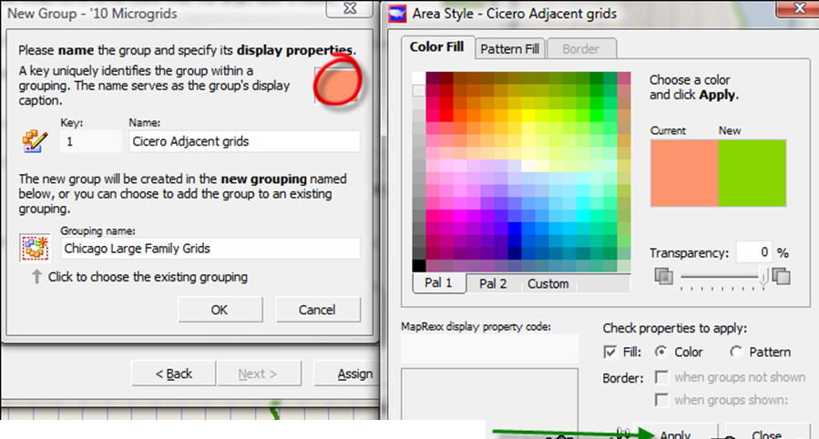
Area Style Selector
Click the orange color panel (red circle) to get the Area Style Selector. Then click whatever color you want to become the new grouped-grid color, and click Apply.
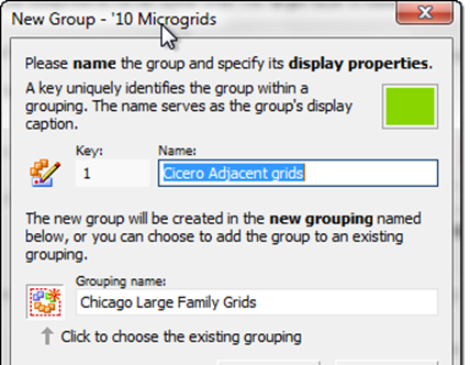
Getting ready for chartreuse MicroGrids
Fill in the Name and Grouping name as in the previous capture.
Now you have a new grouping, group name, and group color. Click "OK".
Finally, click "Assign".
MicroGrids grouping hidden by ZIP grouping
At this point, your map will still show the orange ZIP grouping, and the green Microgrid grouping peeking out behind it. You won't need those two ZIP codes in the map anymore, so you can hide the grouping by clicking the "Hide Groups on Layer" button (red circle above).
Now, with this newly-created inventory of grids falling within these two ZIPs, change the current layer to grids (white arrow), and from the Objects menu choose Object Manager.
Making MicroGrids the current layer
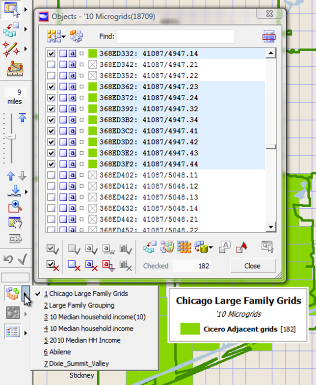
Click Microgrids (above) to make grids the current layer. Then, click the Select by Group button (red circle below), check the Cicero Adjacent grids (green arrow) - there are 182 of them - click the Select button, and they will become green.
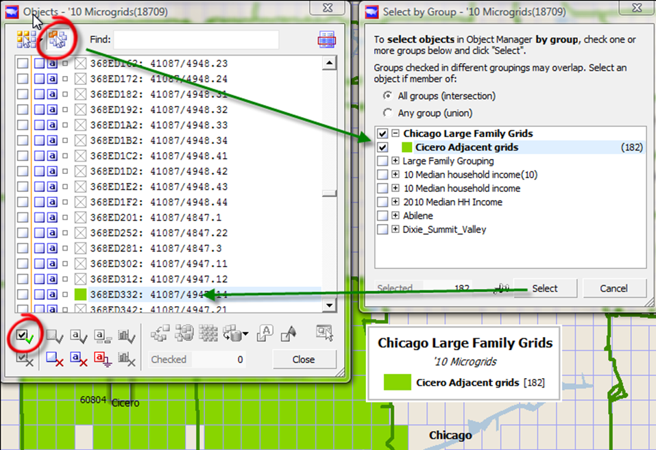
Checking grouped MicroGrids in Object Manager
Finally, above, with the grids selected (green arrow) and the grid names highlighted in blue, check them off (red circle). They are checked! Your Object Manager looks like this:
Export Grouped MicroGrids to Google Earth
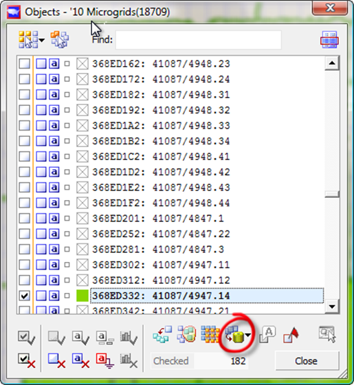
The checked items are the grids within the two ZIPs, and in a moment we will press the "Export Object Data" button (red circle above -- don't press it yet), and choose Locate in Google Earth. Remember Google Earth? But wouldn't it be nice if we were able to see, not the uniform green grids, but the data thematic map that we made earlier? Fortunately with Object Manager, the checks will stay checked while we change the currently displayed grouping.
Changing the current grouping
Click the "Choose grouping to display" arrow-out menu (above) to show the groupings on the Microgrid layer, and noticing that Chicago Large Family Grids is shown, choose the previously grouped "Large Family Grouping" instead. Your map, grouping legend, and Object Manager grid coloring will all change to the orange thematic palette.
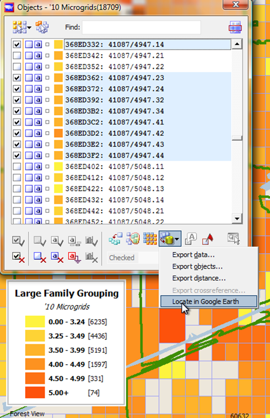
Locate in Google Earth
Choose Locate in Google Earth, and the CHECKED grids will be exported with their orange color, and their data range values, as shown below.
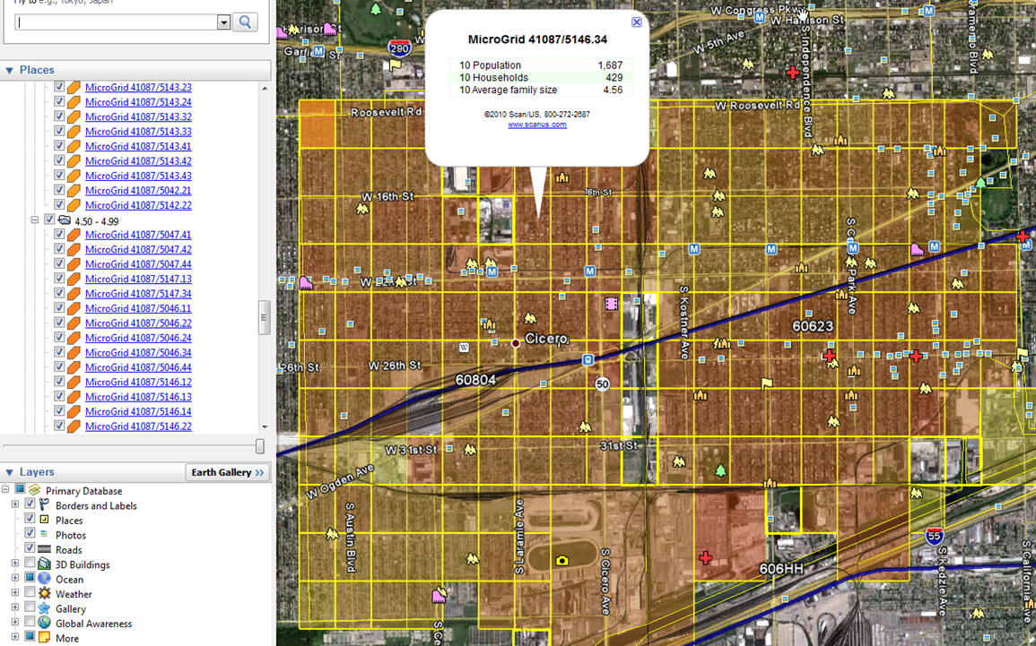
MicroGrid map, with data, in Google Earth
In Google Earth you can zoom in, turn the grids on and off by category and individually, and click on any one of them to see the demographics values that were selected in Quicklook when you exported.
If you want to color in the grids with a different demographic variable such as population density, median income, percent Hispanic, cars per household, or whatever, the grids will remain checked and you can quickly generate a series of thematic maps for Google. In fact, scrolling back up to the next-to-last picture, you will notice an "Export Objects" option - that will create a .kml or .kmz file (at your option) that you can mail to someone else with Google Earth, and on the Data menu, you will find an "Export data.." option to export the data for these grids.